


Abstract
The authors compared five methods of studying survival bias associated with time-to-treatment initiation in a drug effectiveness study using medical administrative databases (1996–2002) from Quebec, Canada. The first two methods illustrated how survival bias could be introduced. Three additional methods were considered to control for this bias. Methods were compared in the context of evaluating statins for secondary prevention in elderly patients post-acute myocardial infarction who initiated statins within 90 days after discharge and those who did not. Method 1 that classified patients into users and nonusers at discharge resulted in an overestimation of the benefit (38% relative risk reduction at 1 year). In method 2, following users from the time of the first prescription and nonusers from a randomly selected time between 0 and 90 days attenuated the effect toward the null (10% relative risk reduction). Method 3 controlled for survival bias by following patients from the end of the 90-day time window; however, it suffered a major loss of statistical efficiency and precision. Method 4 matched prescription time distribution between users and nonusers at cohort entry. Method 5 used a time-dependent variable for treatment initiation. Methods 4 and 5 better controlled for survival bias and yielded similar results, suggesting a 20% risk reduction of recurrent myocardial infarction or death events.
Survival bias occurs in studies that assess the effect of a treatment on survival or any other failure time, when the classification of “exposed” subjects requires that a person survives (or be event free) until the date he/she receives the treatment. Subjects who die shortly after the start of follow-up may not have had an opportunity to become exposed and are “unexposed” by definition. This introduces an artificial survival advantage associated with the exposed subjects regardless of treatment effectiveness. Typically, survival bias arises when a study uses a time window from the start of follow-up to define users of a medication, while subsequent analyses fail to account for the fact that the users' time-to-treatment initiation represents unexposed survival time. The magnitude of this bias depends on the length of the time window and the risk for outcome in this period (1). Treatment effect will be much more distorted if an excessive number of early deaths are classified into the unexposed group and a longer time window captures more late users who, by definition, survive longer.
Some observational studies of drug effectiveness may have failed to recognize and effectively control for survival bias, thereby resulting in biased estimates (2–5). In practice, patients discharged from hospitalization for a severe disease condition, such as acute myocardial infarction (AMI), exacerbation of chronic obstructive pulmonary disease, or asthma, are at high risk of event recurrence or mortality (6). Studies of treatment effectiveness in these patients are prone to survival bias. For example, in a study assessing the effect of use of inhaled corticosteroids on reducing hospital readmission and mortality in patients with chronic obstructive pulmonary disease (2), the authors defined the users as those who filled a prescription in the 90-day period following discharge and nonusers, otherwise. Both groups were followed for 1 year after discharge. The study reported a 26 percent reduction in mortality and hospital readmission associated with inhaled corticosteroids use. However, the benefit may have been overestimated because of survival bias. The higher event rate, likely driven by rehospitalization in the early period following discharge, may have forced a majority of the early events to be classified into the nonuser group, because most of these subjects have not yet had an opportunity to receive the medication. A subsequent analysis in a similar setting using a time-dependent variable for treatment initiation (1) suggested no effect of the treatment (rate ratio = 1.00, 95 percent confidence interval (CI): 0.79, 1.26).
To reduce survival bias, the authors of some studies have used an alternative time 0 for follow-up, such as the time of the first prescription rather than the date of discharge. The difficulty is, however, among nonusers, that there is no actual prescription time of the study drug. Several approaches have been used in the literature to define time 0 for the nonusers. Some authors used a method that randomly assigns a prescription time to the nonusers as time 0 for the follow-up (7), while others chose the prescription time of another drug filled by the nonusers during the same period used to identify the users (8). However, survival bias may still be present in these methods. For example, random assignment of prescription time to nonusers may not lead to equalization of the survival pattern between the two groups, and the survival difference may remain. In the case of using a prescription time of another drug in nonusers, the drug may be associated with the study outcome and confound the treatment effect under study. Finally, the method that dichotomizes subjects into “users” and “nonusers” based on discharge prescriptions causes misclassification. A considerable number of subjects who fill the prescription during the subsequent days are misclassified as “nonusers” (9). This may attenuate the treatment effect toward the null.
Despite the many methods used, there is a lack of an optimal approach that adequately controls for survival bias. The current study was to compare different methods in the control of this bias. We proposed a prescription time-distribution matching method and compared its performance with other methods. We applied these methods in the context of evaluating the effectiveness of statins for secondary prevention in elderly patients post-AMI.
MATERIALS AND METHODS
Data source
Data were from the Quebec, Canada, hospital discharge summary database (Maintenance et exploitation des données pour l'étude de la clientéle hospitalière for Québec, Med-Echo) and the physician and prescription claims databases (the Régie de l'assurance maladie du Québec, RAMQ). Up to 15 diagnoses of comorbidity are recorded in the hospital discharge database. In- and outpatients' physician visits, diagnoses, and prescribed medications are recorded in the physician and prescription claims databases. Prescription information includes type of medication, dosage, quantity, and duration. Death information is available from provincial registry databases. All databases were linked with patients' unique, encrypted, health-care insurance number. Several validation studies have been conducted previously to assess the accuracy of the coding (10–12).
Study cohort
A retrospective cohort was used. Eligible patients were Quebec elderly (≥65 years) who were discharged alive with a diagnosis of AMI between April 1996 and March 2000. Survival data were available for these patients until April 2002.
Inclusion and exclusion criteria
Patients were included if they had an AMI (International Classification of Diseases, Ninth Revision, code 410) coded as their most responsible diagnosis. We excluded patients if they met any of the following exclusion criteria: 1) the AMI was coded as an in-hospital complication; 2) the AMI admission was a transfer from another hospital (this is to avoid counting patients twice, yet all transfers related to the initial AMI admission are counted in the total length of hospital stay); 3) the total length of hospital stay was less than 3 days (this is to exclude ruled-out AMI cases and those admitted only for procedures); 4) the patient was discharged to an institution for long-term care or a rehabilitation center or moved out of the province (as information on medication was not available in these cases); and 5) the health-care number was invalid.
Baseline characteristics
Patients' characteristics included age, sex, and comorbidity at discharge. The latter included coexisting cardiovascular and lung diseases, chronic kidney or liver conditions, and other diseases, such as diabetes, dementia, and malignancy. Concurrent use of β-blockers, angiotensin converting enzyme inhibitors, antiplatelet drugs (aspirin, clopidogrel), calcium channel blockers, diuretics, warfarin, and digoxin was determined. In addition, we obtained information for each patient regarding length of hospital stay, in-hospital procedures (catheterization, percutaneous coronary intervention, coronary artery bypass graft surgery), specialty of the treating physician, and the type of hospital.
Definition of exposure and endpoints
Patients who filled at least one statin prescription less than 90 days after discharge were defined as statin “users.” Patients were nonusers otherwise. The study endpoint was defined as a recurrent AMI or death due to any cause, whichever occurred first. Patients were followed until 1 year postdischarge or the occurrence of a study outcome. In addition, follow-up at 6 months postdischarge and full follow-up (until April 2002) were also studied.
Study methods
We compared five methods (table 1) (appendix figures 1 and 2). The first two methods illustrated how survival bias could be introduced in drug effectiveness studies. Three additional methods were considered to control for this bias, including a newly proposed method using prescription time-distribution matching.
Description of different methods
Time 0 for the follow up | Variable representing statin exposure | Method of analysis | |
|---|---|---|---|
| Method 1: simple grouping | Hospital discharge | Fixed-in-time dummy variable (1 = users; 0 = nonusers) | Cox proportional hazards model |
| Method 2: random selection of prescription time | Users: time of the first prescription; nonusers: randomly selected time between 0 and 90 days | Fixed-in-time dummy variable (1 = users; 0 = nonusers) | Cox proportional hazards model |
| Method 3: follow-up since the end of the exposure time window | Day 90 postdischarge | Fixed-in-time dummy variable (1 = users; 0 = nonusers) | Cox proportional hazards model |
| Method 4: prescription time-distribution matching | Users: time of the first prescription; nonusers: time assigned according to the distribution of users' time of the first prescription | Fixed-in-time dummy variable (1 = users; 0 = nonusers) | Cox proportional hazards model |
| Method 5: time-dependent initiation | Hospital discharge | Time-dependent exposure variable (0 = before use; 1 = after use) | Time-dependent Cox model |
Methods introducing survival bias.
Method 1 (simple grouping) (2).
Statin use is represented by a binary variable, taking the value 1 for those who initiated a statin within 90 days postdischarge and 0 for those who did not. Both groups are followed from the date of discharge until the occurrence of a study endpoint or the end of follow-up. This method defines the users by use of their future exposure. The users' “event-free” person-times before their first prescription inflate the denominator of the event rate in the group and lead to an artificially small rate ratio.
Method 2 (random selection of prescription time) (7).
Statin use is represented by a binary variable, taking the value 1 for those who initiated statins within 90 days postdischarge and 0 for those who did not. The nonusers are assigned a time 0 that is randomly selected between 0 and 90 days postdischarge. Time 0 for a user is the time of his/her first prescription. Nonusers who had an event before the assigned time 0 are excluded from the analysis. Both groups are then followed from time 0 until the occurrence of recurrent AMI, death, or the end of study follow-up. This method results in a uniform distribution of time 0 for the nonusers and likely introduces a survival bias if the distribution of time 0 for users departed largely from the uniform distribution.
Methods to control for survival bias.
Method 3 (follow-up begins at day 90).
Statin use is represented by a binary variable, taking the value 1 for those who initiated a statin within 90 days postdischarge and 0 for those who did not. Users and nonusers of statins are followed from the end of the exposure time window (i.e., 90 days postdischarge) until the occurrence of recurrent AMI, death, or the end of study follow-up. This method controls for survival bias by following only 90-day survivors from the same point in time after discharge.
Method 4 (prescription time-distribution matching).
Statin use is represented by a binary variable (1 for users and 0 for nonusers). The number of days from discharge to the dispensing time of the first prescription is assessed for the users. For each nonuser, a time 0 is selected at random from this set and assigned to him/her. Therefore, the overall distribution of time 0 of the nonusers is matched to that of the users' time of first prescription (time 0). This avoids the imbalance of the prescription time distribution between the two groups, which leads to survival bias in method 2. Both groups are followed from time 0 until the occurrence of recurrent AMI, death, or the end of study follow-up. Nonusers who had an event before the assigned time 0 are excluded from the analysis.
Method 5 (time-dependent variable for treatment initiation) (1, 13).
A time-dependent variable for statin initiation is used to define current users and nonusers. Follow-up starts at discharge until the earliest of recurrent AMI, death occurrence, or the end of study follow-up. For users, the value of the time-dependent variable is 0 before the time of first statin prescription and changes to 1 when the prescription is filled and onward. For the nonuser, the value remains as 0 in the follow-up. This method accurately represents the exposure status and classifies the “event-free” person-time of the users before their first prescriptions as the unexposed follow-up time.
Statistical analysis
Descriptive analyses were used to compare patient characteristics at discharge between statin users and nonusers. The rates of recurrent AMI and mortality were determined during the 1-year follow-up after discharge. A multivariate Cox proportional hazards model (14) was used to analyze the time to recurrent AMI or death in all methods, except that, in method 5, a time-dependent Cox regression model variable was used. For each method, an adjusted hazard ratio was reported for recurrent AMI or death during the 1-year postdischarge period. In secondary analysis, adjusted hazard ratios for outcomes at the 6-month and full follow-up periods were reported.
Comparison of the methods
The five methods were compared to determine 1) the differences in point estimates of the adjusted hazard ratios and the width of 95 percent confidence intervals, 2) the statistical efficiency in terms of the number of subjects excluded from the analysis, and 3) additional advantages and limitations in applications.
All analyses were conducted by use of SAS, version 8.0, software (SAS Institute, Inc., Cary, North Carolina). A significance level of 0.05 (two sided) was used for all tests.
RESULTS
The cohort included 21,521 elderly patients who met the inclusion criteria. Among them, 6,235 patients (29 percent of the cohort) filled a statin prescription during the first 90 days after discharge. The median follow-up time of the cohort was 3.0 years (25th–75th percentile: 1.6–4.4 years).
We observed that users and nonusers differed in several baseline characteristics (table 2). Overall, users appeared to be younger and had less comorbidity than did nonusers.
Characteristics of statin users and nonusers at discharge from a hospitalization for acute myocardial infarction, Quebec, Canada, 1996–2002
Characteristics | Users | Nonusers |
|---|---|---|
| No. of patients | 6,235 | 15,286 |
| Median age (years) | 72 (68–76)* | 76 (70–81) |
| Males (%) | 60 | 56 |
| Baseline comorbidities (%) | ||
| Hypertension | 36 | 33 |
| Diabetes | 23 | 25 |
| Congestive heart failure | 20 | 28 |
| Cardiac dysrhythmia | 17 | 20 |
| Chronic obstructive pulmonary disease | 16 | 21 |
| Cerebrovascular disease | 7 | 8 |
| Chronic renal failure | 7 | 10 |
| Malignancy | 2 | 3 |
| Dementia | 1 | 3 |
| Hyperlipidemia | 52 | 10 |
| In-hospital procedures (%) | ||
| Catheterization | 40 | 22 |
| Percutaneous coronary intervention | 19 | 10 |
| Coronary artery bypass graft surgery | 8 | 5 |
| Cardiac medications (prescriptions at discharge) (%) | ||
| Nitrates | 54 | 53 |
| Beta-blockers | 52 | 38 |
| Angiotensin converting enzyme inhibitors | 35 | 33 |
| Antiplatelet agents† | 48 | 43 |
| Diuretics | 19 | 27 |
| Calcium-channel blockers | 17 | 17 |
| Warfarin | 11 | 11 |
| Digoxin | 10 | 14 |
| Specialty of treating physicians (%) | ||
| Cardiologist | 48 | 44 |
| Internist‡ | 11 | 9 |
| General practitioner and other specialists | 40 | 45 |
| Hospital characteristics (% of patients treated) | ||
| Teaching hospital | 18 | 14 |
| Catheterization availability | 30 | 26 |
| Hospital in rural location§ | 5 | 5 |
| Median length of hospital stay (days) | 9 (7–15) | 10 (7–15) |
Numbers in parentheses, 25th–75th percentile interquartile range.
Antiplatelet agents include aspirin and clopidogrel.
Internist excluding cardiologist.
Rural location: with 0 in the middle of the first 3 digits of the postal code (defined by Census Canada).
Time to first statin prescription and statin use
The 90-day exposure time window captured 92 percent of all first post-AMI statin prescriptions during the first year. The distribution of time of the first statin prescription was skewed (median: 1 day; 25th–75th percentiles: 0–24 days). Close to one half of all the prescriptions (n = 3,075) were dispensed at discharge, and 81 percent were dispensed within the first month. One-year adherence (defined as the ratio of total number of supplied days of statin prescriptions during 1 year divided by 365 days) was high among users of statins (median: 0.95; 25th–75th percentiles: 0.87–1.00).
Risk of recurrent AMI and mortality within the first year postdischarge
By the end of 1 year, 4,168 subjects (19 percent of all subjects) had a recurrent AMI or death. Among them, 1,930 subjects (46 percent) had their first event during the first 90 days postdischarge, which coincided with the time window used to define users. The event rate peaked during the first 30 days, when it reached 1.1–1.3 per 1,000 patient-days. It then decreased to about 0.6–0.7 per 1,000 patient-days by 90–100 days after discharge and remained stable thereafter (figure 1)
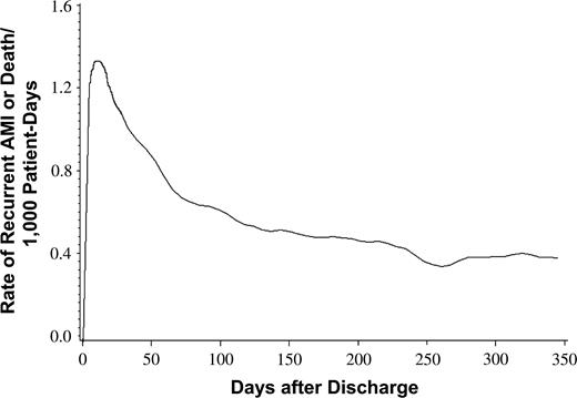
Rate of recurrent acute myocardial infarction (AMI) or death during the first year after hospital discharge, Quebec, Canada, 1996–2002.
Results from different methods evaluating statin effectiveness
In method 1 (simple grouping), statin use appeared to reduce the risk of recurrent AMI or death by 38 percent (adjusted hazard ratio (HR) at 1 year postdischarge = 0.62, 95 percent CI: 0.55, 0.69). The effect was overestimated, because the design and analysis introduced an artificial survival advantage to the users. A total of 254.4 person-years, representing users' survival time since discharge to their first prescription, were misclassified as exposed person-time. These “event-free” person-times inflated the denominator of the event rate in the user group and led to an artificially small rate ratio.
In method 2 (random selection of prescription time), simple random assignment of prescription time to the nonusers gave rise to a uniform distribution of time 0, with a median of 45 days. A total of 1,018 (6.7 percent) nonusers were excluded because of having had an event before their assigned time 0. The method showed that statin use was associated with a marginal, nonsignificant, beneficial outcome (adjusted HR = 0.90, 95 percent CI: 0.80, 1.01). However, because of the uniform distribution of time 0, nonusers had on average longer survival time than did users. The bias was induced by the combination of 1) systematic difference in the time to first prescription between users and nonusers and 2) the substantial change in the absolute level of risk during the first 90 days. The median time 0 of 45 days indicated that half of the nonusers survived and were followed after 45 days postdischarge when the risk of recurrence was lower than that immediately after discharge, whereas half of the users were followed since day 1 (users' median time of first prescription) when the risk was highest. As a result, the nonusers who remained in the study were by design at lower risks for outcomes.
In method 3 (follow-up begins at 90 days), following patients from the end of the 90-day time window led to the exclusion of 294 (4.7 percent) users and 1,622 (10.6 percent) nonusers who had an event in this period. Statin use was associated with a 22 percent reduction of recurrent AMI or death (adjusted HR = 0.78, 95 percent CI: 0.67, 0.90). However, because of exclusion of a large number of events, this method suffered a loss of study information and statistical efficiency.
In method 4 (prescription time-distribution matching), after matching on the prescription time distribution between user and nonuser groups, 364 (2.4 percent) nonusers were excluded because of having an event before their assigned time 0. The estimated risk reduction for recurrent AMI or death associated with statin use was 20 percent (adjusted HR = 0.80, 95 percent CI: 0.72, 0.89). The point estimate was very close to that of method 3, but the confidence interval was narrower, indicating a better precision. Compared with the method using random selection of prescription time, time-distribution matching at study entry achieved similarity in survival patterns between users and nonusers.
In method 5 (time-dependent exposure), a time-dependent representation of statin initiation avoided misclassification of users' survival time before first prescription as the exposed follow-up time. No subject was excluded from the analysis. This method showed that statin use reduced the risk of recurrent AMI or death by 20 percent (adjusted HR = 0.80, 95 percent CI: 0.73, 0.89). This estimated hazard ratio and the 95 percent confidence interval were the same as those estimated from method 4, and the hazard ratio reduction was significantly smaller than that from method 1 of simple grouping (nonoverlapping 95 percent CI).
Overall, the method of simple grouping (method 1) overestimated the benefit, whereas the method of random assignment of prescription time (method 2) attenuated the estimate toward the null. The other three methods (methods 3–5) appeared to be effective in controlling for the bias and provided similar results. This pattern of estimates from different methods was not limited to the outcome by 1 year. A similar pattern was observed in outcomes at 6 months and full follow-up (table 3).
Adjusted hazard ratios* of statin use for recurrent acute myocardial infarction or mortality, Quebec, Canada, 1996–2002
Hazard ratio (95% confidence interval) at 1 year† | Change in hazard ratio relative to method 4 or 5‡ | Hazard ratio (95% confidence interval) at 6 months | Hazard ratio (95% confidence interval) at full follow-up§ | |
|---|---|---|---|---|
| Method 1¶: simple grouping | 0.62 (0.55, 0.69) | −0.23 | 0.58 (0.50, 0.66) | 0.68 (0.63, 0.72) |
| Method 2: random assignment of prescription time | 0.90 (0.80, 1.01) | 0.13 | 1.01 (0.87, 1.17) | 0.80 (0.74, 0.86) |
| Method 3: follow-up begins at day 90 | 0.78 (0.67, 0.90) | −0.03 | 0.93 (0.75, 1.16) | 0.75 (0.69, 0.81) |
| Method 4: prescription time-distribution matching | 0.80 (0.72, 0.89) | 0.84 (0.74, 0.98) | 0.76 (0.71, 0.81) | |
| Method 5: time-dependent exposure | 0.80 (0.73, 0.89) | 0.86 (0.76, 0.98) | 0.76 (0.71, 0.81) |
Multivariate Cox regression model adjusted for demographic and clinical characteristics, procedure, medication use, physician, and hospital type.
Follow-up time since discharge.
Relative change in the adjusted hazard ratio (HR) calculated as follows: (HR of a given method – HR of method 4)/HR of method 4.
Median follow-up of 3.0 years (25th–75th percentile: 1.6–4.4 years).
For descriptions of the respective methods, refer to table 1 and corresponding comments in Materials and Methods.
DISCUSSION
We have demonstrated that survival bias occurs in the study of treatment effectiveness and that its impact on the results is substantial. In the present study, artificial survival advantage associated with either users (in method 1: simple grouping) or nonusers (in method 2: random selection of prescription time) distorted the results. The same data analyzed by methods 3–5, which better controlled for the bias, suggested that statin use was associated with 20–22 percent hazard reduction. This is very different from either a 38 percent reduction or a statistically nonsignificant 10 percent reduction as estimated, respectively, by the first two methods.
Bias due to “survival” in epidemiology
Bias resulting from the subjects' survival is not uncommon in clinical epidemiology. In cross-sectional studies of patients who had rapidly progressing illnesses, a person's survival affects his/her probability of being included in a study (length bias sampling) (15, 16), whereas in the current study of treatment effectiveness, a person's survival affects his/her probability of becoming exposed. Similarly, in the study of cancer recurrence and mortality, the role of “late recurrence” as a predictor for longer survival could be misinterpreted, if one ignores the fact that, to have a late recurrence, a patient has to survive a longer period of time (17–19). Another example, from the transplantation literature, is the duration of waiting time a patient has lived before transplantation. This length of time should not be interpreted as the effectiveness of transplantation to improve survival (20). From these perspectives, the survival bias characterized here is not new. The occurrence of this bias can also be characterized in a more general situation where subjects' survival affects the classification of two comparison groups.
Performance of different methods
The methods we evaluated had three different types of time 0: first, the time of discharge (methods 1 and 5); second, the time of first statin prescription (methods 2 and 4); and third, the time at the end of the exposure time window (method 3). The occurrence of survival bias associated with misclassification of survival time is possible only when using the time of discharge as time 0, because it precedes the time of the first prescription. Unless the prescription is filled on the date of discharge, a subject is unexposed and should be considered as such until the day he/she fills the prescription. This was ignored in method 1 that involved simple grouping. Such misclassification is reduced by using a time-dependent variable for treatment initiation (method 5) or by starting the follow-up at the time of first prescription (methods 2 and 4) or the time when all the first prescriptions have occurred, as specified by the design (method 3), here, the end of the 90-day time window.
However, using the time of first prescription as the study entry may still introduce survival bias through selection. In the method of random selection of prescription time (method 2), the uniform distribution led to the inclusion of a large proportion of nonusers' having an assigned time 0 late in time compared with users. Furthermore, because the risk for outcome decreased considerably over time, the nonusers appeared to have an overall lower risk than did the users. This differential selection does not occur in the distribution matching design (method 4), where the proportion of subjects starting at different points in time in the 90 days was similar between users and nonusers. Similarly, there was no “imbalance” in survival time, when the subjects were all followed from the same point in time (method 3).
Compared with other methods, the time-dependent approach (method 5) showed several advantages. First, with regard to statistical efficiency, no subject was excluded from the analysis, whereas this number was 1,916 and 364 in method 3 (follow-up since day 90) and method 4 (prescription time-distribution matching), respectively (table 4). The substantial exclusion also raises the concern of limited generalizability. For example, in method 3, the results may apply only to those 90-day survivors in the study. Second, the time-dependent method has the advantage of providing effect estimation at any time point after discharge, as a subject is allowed to be in the risk set as a nonuser early on and becomes a user later. In other methods, treatment effect estimation is not available or reliable for the initial time period when “users” are still being defined.
Comparison of different methods in the control of survival bias, Quebec, Canada, 1996–2002
Source of bias | Study efficiency (no. excluded) | Advantages | Limitations | |
|---|---|---|---|---|
| Method 1: simple grouping | Bias introduced by misclassification of unexposed follow-up of users before treatment initiation | 0 | Overestimation of treatment effect | |
| Method 2: random assignment of prescription time | Bias introduced by preferential selection of nonusers with longer survival and underlying risk change | 1,018 nonusers | Treatment effect biased toward the null; loss of statistical efficiency and precision | |
| Method 3: follow-up begins at day 90 | Bias controlled by limiting to patients who survived 90 days | 294 users; 1,622 nonusers | Major loss of study information, efficiency, and precision; effect during the first 90 days ignored; and large exclusion results in limited generalizability | |
| Method 4: prescription time-distribution matching | Bias controlled by selecting patients with a similar survival pattern | 364 nonusers | No apparent loss of study efficiency; useful when comparing users only (e.g., early vs. delayed use) | Effect estimation not available during the period when users are being defined; assumption that the prescription will occur at random unlikely to be met |
| Method 5: time- dependent initiation | Bias controlled by classifying patients as nonusers until they filled a prescription | 0 | Best statistical efficiency; allows effect estimation at any point in time after discharge | Comparison is limited to use vs. no use; assumption that the prescription will occur at random unlikely to be met |
Despite these advantages, the time-dependent method relies on additional assumptions. The time-dependent representation of statin initiation usually implies that the first prescriptions occur at unpredictable (random) times (21). This assumption is difficult to assess in this case, as the physician's decision to prescribe statins may be influenced by the severity of a patient's condition and life expectancy. Physicians may withhold statins from patients until their condition becomes stable. Thus, receiving a statin may indicate a lower risk status independent of the treatment effect of statins. In such case, survival bias remains. Similarly, this assumption also affects the ability of the method of prescription time-distribution matching (method 4) to control for survival bias, because the matching is based on the observed pattern of prescription time, hence, the survival time.
Notably, methods 4 and 5 provided almost the same estimates and 95 percent confidence intervals, suggesting their similar effectiveness in the control of survival bias. An advantage associated with method 4 is that it is useful where the comparison is made among users only, for example, in studying the effect associated with the timing of treatment initiation (early vs. delayed initiation). Survival bias is possible, because the two groups differ systematically in the time of treatment initiation. The time-dependent approach used to compare use versus no use will have limited application in this case.
Effectiveness of statins in elderly patients post-AMI
Despite the control for survival bias, the estimated treatment effect of statins is still susceptible to other common biases in observational studies, especially confounding by indication (22). In practice, statins are prescribed more to patients perceived to experience the benefit (23). Older patients and patients with severe coexisting diseases are less likely to receive statin prescriptions. Despite adjustment for a wide spectrum of characteristics, it is possible that we cannot control for all the factors that may affect a physician's decision to prescribe a statin or not. Therefore, even after control for survival bias, our results should still be interpreted with caution.
Conclusion
We have shown that effective control for survival bias relies on correct use of study design and analysis. Our empirical assessment using real-life data suggests that the methods of prescription time-distribution matching and time-dependent variable for treatment initiation exhibit better performance and give very similar results. This is determined by their control for survival bias, statistical efficiency, and advantages in application.
APPENDIX
Study Designs
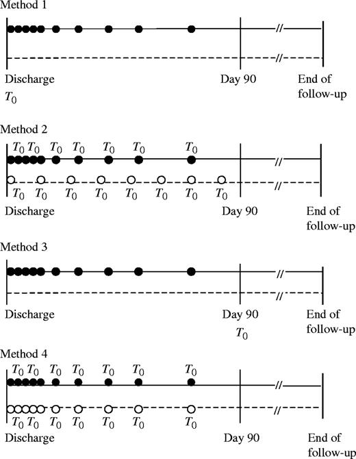
Study designs in methods 1–4. Method 1: simple grouping; method 2: random selection of prescription time among nonusers; method 3: follow-up since the end of exposure time window; method 4: prescription time-distribution matching between users and nonusers. Solid line, follow-up of user group; dashed line, follow-up of nonuser group. T0, time 0 for follow-up. Black circles, users' time of first statin prescription; white circles, nonusers' assigned time of first statin prescription.
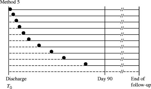
Study design in method 5: time-dependent variable for treatment initiation. Solid line, unexposed person-time; dashed line, exposed person-time. T0, time 0 for follow-up. Black circle, users' time of first statin prescription.
This study was funded in part by a grant from the Canadian Institutes of Health Research (grant ATF-66669). Dr. Zhou was supported by a scholarship from the Natural Science and Engineering Research Council of Canada and a fellowship from the Canadian Cardiovascular Outcome Research Team. Dr. Rahme is a research scholar funded by the Arthritis Society. Drs. Pilote and Abrahamowicz are research scholars funded by the Canadian Institutes of Health Research.
Conflict of interest: none declared.
References
Suissa S. Effectiveness of inhaled corticosteroids in chronic obstructive pulmonary disease: immortal time bias in observational studies.
Sin DD, Tu JV. Inhaled corticosteroids and the risk of mortality and readmission in elderly patients with chronic obstructive pulmonary disease.
Sin DD, Tu JV. Inhaled corticosteroid therapy reduces the risk of rehospitalization and all-cause mortality in elderly asthmatics.
Soriano JB, Kiri VA, Pride NB, et al. Inhaled corticosteroids with/without long-acting beta-agonists reduce the risk of rehospitalization and death in COPD patients.
Donahue JG, Weiss ST, Livingston JM, et al. Inhaled steroids and the risk of hospitalization for asthma.
Hunninghake DB. Postdischarge lipid management of coronary artery disease patients according to the new National Cholesterol Education Program guidelines.
Mamdani M, Rochon PA, Juurlink DN, et al. Observational study of upper gastrointestinal haemorrhage in elderly patients given selective cyclo-oxygenase-2 inhibitors or conventional non-steroidal anti-inflammatory drugs.
Ray WA, Stein CM, Daugherty JR, et al. COX-2 selective non-steroidal anti-inflammatory drugs and risk of serious coronary heart disease.
Aronow HD, Topol EJ, Roe MT, et al. Effect of lipid-lowering therapy on early mortality after acute coronary syndromes: an observational study.
Kennedy CC, Brien SE, Tu JV. An overview of the methods and data in the CCORT Canadian Cardiovascular Atlas project.
Levy AR, Tamblyn RM, Fitchett D, et al. Coding accuracy of hospital discharge data for elderly survivors of myocardial infarction.
Humphries KH, Rankin JM, Carere RG, et al. Co-morbidity data in outcomes research: are clinical data derived from administrative databases a reliable alternative to chart review?
MacDonald TM, Wei L. Effect of ibuprofen on cardioprotective effect of aspirin.
Wolfson C, Wolfson DB, Asgharian M, et al. A reevaluation of the duration of survival after the onset of dementia.
Correa JA, Wolfson DB. Length-bias: some characterizations and applications.
Dancourt V, Quantin C, Abrahamowicz M, et al. Modeling recurrence in colorectal cancer.
Fredriksson I, Liljegren G, Arnesson LG, et al. Local recurrence in the breast after conservative surgery—a study of prognosis and prognostic factors in 391 women.
Diez M, Pollan M, Muguerza JM, et al. Time-dependency of the prognostic effect of carcinoembryonic antigen and p53 protein in colorectal adenocarcinoma.
Jamieson SW, Stinson EB, Shumway NE. Cardiac transplantation in 150 patients at Stanford University.
Allison PD. Time dependent covariates. Survival analysis using the SAS system: a practical guide. Cary, NC: SAS Institute, Inc,
Salas M, Hofman A, Stricker BH. Confounding by indication: an example of variation in the use of epidemiologic terminology.

